Glacier Simulator#
The glacier simulator is an interactive web application with which you can learn (and teach) about glacier flow, how glaciers grow and shrink, what glacier properties influence their size or velocity, and a lot more!
You can start the app by clicking on this link: ![]()
Note
The glacier simulator app runs a numerical glacier model in the background, using computer resources on the cloud. If several people are using the app at the same time, the server might become slow or unresponsive. In this case, we recommend to use the app on MyBinder or even locally on your own computer (see Launching from Docker below).
Getting started with the app#
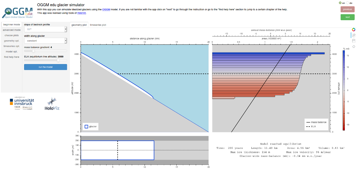
The upper panel in the app is a guided tutorial about the app’s functionalities. You can navigate it with the “Next” and “Previous” buttons, or use the “Find help here” overview.
Questions to explore with this app#
With this app, you can address many questions, by yourself or in class! This list will grow in the future (documentation takes time!).
Glacier shape#
See antarcticglaciers.org (mass-balance) for an introduction about glacier mass-balance and the ELA, or our Introduction to glaciers graphics for an illustration.
Experiment:
In “Beginner mode”, start by setting the ELA to 3000m a.s.l, and note on a piece of paper: the equilibrium volume of the glacier, its length and maximal thickness.
Now choose the “Wide top, narrow bottom” glacier shape and run the model again.
Question to answer:
Is the new glacier longer or shorter than before? Why?
Take home messages
A glacier with a wider top has a larger accumulation area. It can therefore accumulate more mass (more ice) in the upper part. The glacier can flow further down until melt rates become large enough to compensate for this additional ice.
Take home messages (advanced)
An additional (and more advanced) observation can be done by looking at the “Accumulation Area Ratio” (AAR) of the two glaciers. In the “constant width” case, the glacier area is the same above and below the ELA (equilibrium AAR = 0.5, only true if the mass-balance gradient is also constant). In the “wider-top” case, the AAR at equilibrium is larger than 0.5: indeed, by flowing further down valley, the glacier is loosing more mass at its terminus than at its head, albeit over a different area (width). See our AAR (Accumulation Area Ratio) experiments to learn more about the AAR.
Equilibrium Line Altitude (ELA)#
See antarcticglaciers.org (mass-balance) for an introduction about glacier mass-balance and the ELA, or our Introduction to glaciers graphics for an illustration.
We are going to show that the ELA is determinant in shaping glaciers.
Experiment:
In “Beginner mode”, start by setting the ELA to 2500m a.s.l, and note on a piece of paper: the equilibrium volume of the glacier, its length and maximal thickness.
Now change the ELA up to 3500m a.s.l in 200m increments and, at each step, note the equilibrium volume of the glacier, its length and maximal thickness.
Next draw these variables on a graph, as a function of the ELA.
Questions to answer:
How does glacier volume change with ELA? Can you explain why?
What about glacier length and thickness?
Are these changes linear, or more complex?
Take home messages
An example graphic that students could come up with by varying the ELA with different shapes:
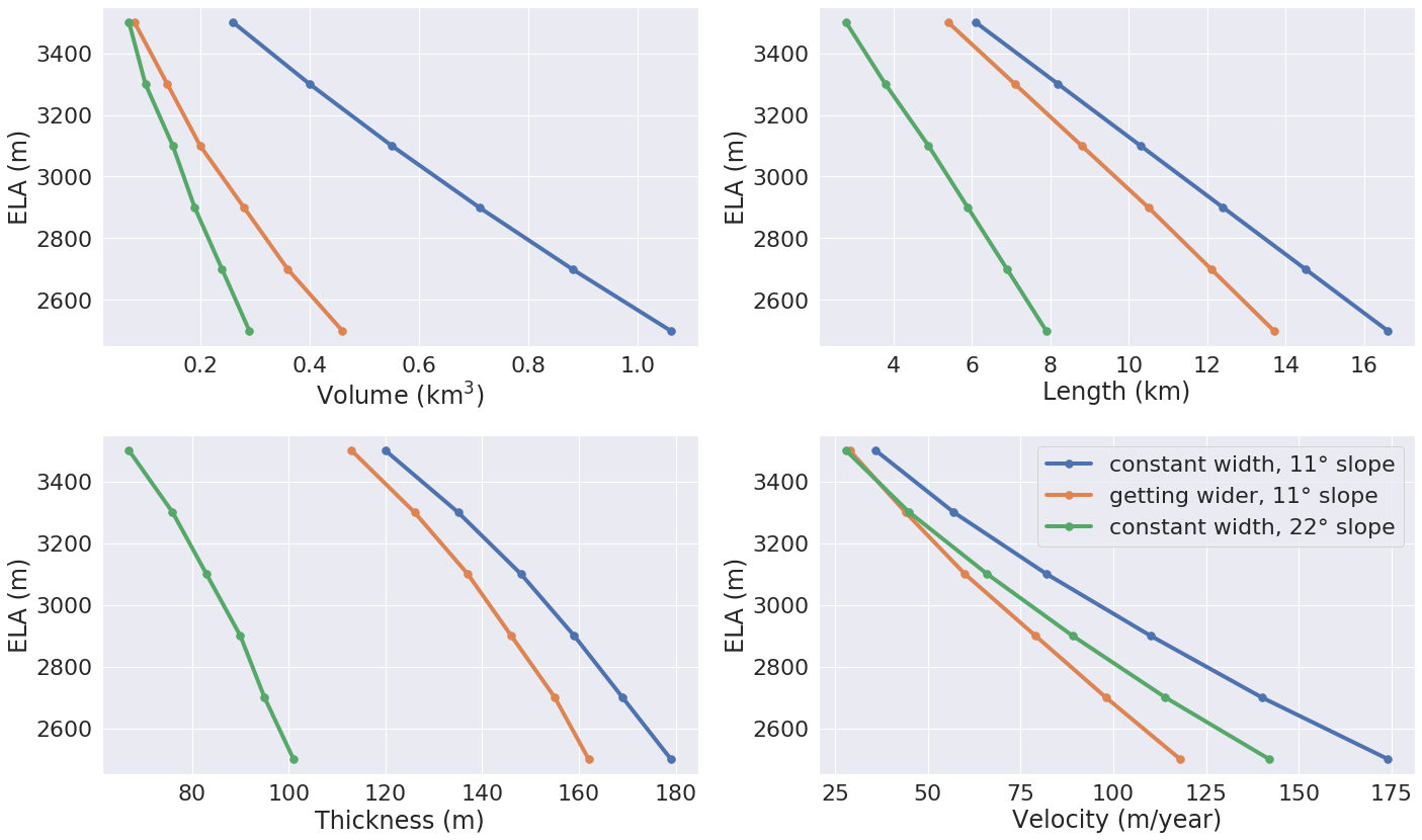
The lower the ELA, the larger the equilibrium glacier. The length, volume or maximal thickness are not necessarily linear functions of the ELA: these depend on the physical relationships between ice flow and slope, as well as the feedback between glacier elevation and mass-balance.
Glacier slope#
The slope of a glacier bed is one key ingredient which determines glacier flow. For an introduction, visit antarcticglaciers.org (glacier-flow). In short: glaciers flow downslope driven by the gravitational force. This force can be decomposed into an along-slope component and perpendicular to the slope component (see this illustration in wikipedia). The along-slope component “pulls” the glacier downwards and the perpendicular component “flattens” the glacier.
Experiments:
Beginner:
Use beginner mode with standard settings (constant width, mass balance gradient of 4 and ELA of 3000) and run the model with all different settings for the slope and use the geometry plot for inspection.
Take note on a piece of paper of the ice thickness, volume, area and length at the end of each model run.
Advanced:
Conduct the same experiment as for Beginner, but additionally take notes of the velocity and look how the parameters change with time in the timeseries plot.
Questions to answer:
Beginner:
Which glaciers are thicker? Steep or flat ones? And why?
Advanced:
Which glaciers are faster? Steep or flat ones? How and why does the velocity change with time?
Take home messages
glaciers flow downslope under gravity
the steeper the slope the thinner the glacier (larger along-slope gravitational force)
the flatter the slope the larger the equilibrium velocity. When the glacier is thin (has not much mass) the along-slope component is more important. When the glacier is getting thicker the perpendicular component is getting more weight. This partly explains slower velocities for flatter slopes at the start of the model run, and higher velocities when the glacier is getting thicker. For steeper slopes the velocities at the start are large and so more ice is transported downwards, and the glacier stays relatively thin.
Surging glaciers#
Some of the world’s glaciers experience “surges” during which they flow much faster than usual and can advance dramatically. For an introduction see antarcticglaciers.org (surging-glaciers) , or this video of surging Karakorum glaciers seen from space.
We will use the simulator app to explore the characteristics of a surging glacier.
Experiment:
Use the “beginner mode” with standard settings (constant width, mass balance gradient of 4 and ELA of 3000) and run the model to create a glacier in equilibrium.
This glacier should now experience a surge which lasts for ten years: Switch into the “advanced mode”. Turn on “sliding”, i.e. the glacier will “slip” on the bedrock, and let the model advance for 10 years.
Between surge events long periods of quiescence happen: simulate one by advancing your glacier without sliding for 100 years.
Repeat the surge event and the period of quiescence. Use the timeseries plots and the timeseries options to show the maximum velocity as well as the maximum thickness.
Questions to answer:
Beginner:
During a surge event: How much faster is the glacier during a surge in comparison to a “normal” (quiescence) period? How much gains the glacier in length?
After a surge event: How can you explain the glacier retreat?
Advanced:
Why is the glacier thinning during a surge?
How can you explain the opposing behaviours of length and volume during a surge?
Why is the glacier thickening after the surge?
Take home messages
During a surge event: The glacier flows faster and reaches lower in the valley. In the upper parts the accumulation of snow does change, but not much (accumulation is slightly less since the glacier is thinner: a process called mass-balance / elevation feedback). At the same time, a much larger area than usual of the glacier is exposed to melt below the ELA. Therefore the glacier thins and looses volume, although it is still advancing.
After a surge event: The glacier flow recovers its usual “slow” velocity. The glacier will retreat until it accumulated enough ice to advance again.
Going further:
In the notebook surging glaciers you can use OGGM to simulate surging events in Python yourself.
Velocity and thickness along the glacier#
Experiments:
Beginner:
Use “Beginner mode” to simulate a glacier in equilibrium with Width = Constant, ELA = 3000, Mass-balance gradient = 4 and Slope = 11°.
Advanced:
Use “Beginner mode” to simulate a glacier with Width = Wide top, narrow bottom, ELA = 3500, Mass-balance gradient = 4 and Slope = 11°.
Questions to answer:
Beginner:
Make a guess as to where the ice velocity along the glacier is largest?
When you made your guess, go to “Geometry opt.” and tick the box Ice velocity (top left) and Ice thickness (bottom left). Now the red/blue colors are showing the velocity/thickness distribution along the glacier. Did you guess correctly?
Advanced:
What is the influence of the glacier bed bottleneck (narrowing) on ice thickness and velocity? Why?
Take home messages
Beginner:
mass is accumulated from the top of the glacier down to the ELA (areas of positive mass-balance): all this mass must be transported downwards, and so the ice flux at equilibrium is largest at the ELA. Larger ice flux means thicker ice and faster glacier flow.
below the ELA, mass is constantly ablated and the ice flux decreases: lower ice flux means thinner ice and reduced glacier flow velocity.
Advanced:
a narrowing of glacier widths means that the same amount of ice needs to be transported through a smaller door: this means that we have both the creation of a “traffic jam” (thickening) and an increase of ice velocity in order to transport more mass downwards.
in this case, the maximum velocity is no longer located around the ELA but further down (at the bottleneck)
Mass-balance gradient#
See antarcticglaciers.org (mass-balance) for an introduction about glacier mass-balance and the mass-balance gradient.
In short: The climatic regime determines the glacier mass-balance gradient. Discovering global glacier locations using the World Glaciers Explorer reveals that glaciers can be found in quite different climates around the world. Here, we will now discover how different mass-balance gradients are shaping glaciers.
Experiments:
First, simulate a glacier in a maritime climate in temperate latitudes (larger mass-balance gradient, e.g. 10). For this, use the “Beginner mode” (ELA = 3000, Width = Constant and Slope = 11°) and let the glacier grow until it reaches equilibrium and note on a piece of paper: the equilibrium Time, Length, Area, Volume, Max ice thickness and Max ice velocity of the glacier.
Next, simulate a glacier in a continental climate in polar latitudes (lower Mass Balance gradient, e.g. 3) and take some notes again.
Questions to answer:
Beginner:
Which of the two glaciers (maritime or continental) is thicker (Max ice thickness)?
Which is flowing faster (Max ice velocity)?
Which reaches the equilibrium faster (Time)?
Advanced:
How are Length, Area and Volume affected?
Take home messages
the larger the mass-balance gradient, the larger the accumulation of mass (ice) at the top
more accumulation leads to a thicker glacier and a larger downslope component of the gravitational force (see the Glacier slope experiment)
this larger force causes a larger ice flux and a larger ice velocity
the larger the ice velocity the faster ice is transported downwards and the faster the equilibrium is reached
length and area are not much affected due to the unchanged linear mass-balance profile: no matter which gradient is selected, the total ice gain/loss at a certain height is only determined by the distance away from the ELA (e.g. the same amount of mass is accumulated 100 m above the ELA as there is mass ablated 100 m below the ELA, with a constant width)
whereas the volume is increasing with a increasing mass-balance gradient due to a larger ice thickness
AAR (Accumulation Area Ratio)#
The AAR is the ratio of the accumulation area (= area above the ELA) to the total glacier area (see antarcticglaciers.org (mass-balance)). In this experiment we will have a look at the equilibrium (or balanced) AAR (AAR-eq) and the transient (or annual) AAR (AAR-t). Let’s make some experiments to see what the AAR can tell us about glaciers. For the interpretation of the experiments, note that the total ice gain/loss at a certain elevation equals the mass-balance (black line in top right figure) times the area (i.e., width) at the same elevation. This is important!
Experiments:
Beginner:
Use “Beginner mode” and conduct runs with Width = Constant and Width = Wide top, narrow bottom, and note down the different AAR-eq (ELA = 3300, Mass-balance gradient = 4, Slope = 11°).
Advanced:
Conduct experiments with Constant width and different mass-balance gradients (e.g. Mass-balance gradient below ELA = 4, Mass-balance gradient above ELA = 2 and vice versa) in “Advanced mode”. Note down the different AAR-eq.
Questions to answer:
Beginner:
Explain the observed AAR-eq for Constant width and for Wide top, narrow bottom.
- For Constant width, what values of AAR-t (below or above 0.5) do you expect for an
advancing and a retreating glacier? Can you confirm by looking at the AAR during the simulation, or using the timeseries plots.
Advanced:
How is AAR-eq changing with a different mass-balance gradients below and above the ELA?
- What can you conclude from the experiments about real-world glaciers which have a typical AAR-eq
between 0.5 and 0.8? (see for example Hawkins, 1985)
Take home messages
Beginner:
In the Constant width case and a linear mass-balance, the AAR is around 0.5.The total ice gain/loss at a certain height is only determined by the distance away from the ELA (e.g. the same amount of mass is accumulated 100 m above the ELA as there is mass ablated 100 m below the ELA) and so the glacier area above the ELA equals the glacier area below (approximately).
In the Wide top, narrow bottom case and a linear mass-balance, the AAR is around 0.6. In this case the total ice gain/loss at a certain height is not only determined by the distance away from the ELA but also from the width at a certain height (e.g. if the width 100 m above the ELA is double the width of 100 m below the ELA, so the total ice gain is double of the total ice loss at 100 m from the ELA). In this case the glacier length is longer compared with the case of constant width and in the lower altitudes the more negative mass-balance leads to more ice melt. Overall, the ablation area (area below ELA) stays smaller than the accumulation area, even with a longer glacier.
For an advancing glacier with constant width the AAR-t is well above 0.5 (mass gain), and in the retreating case well below 0.5 (mass loss).
Advanced:
With a mass-balance gradient below the ELA twice the gradient above the ELA, the total ice loss is twice the total ice gain going the same distance away from the ELA. Therefore, the ablation area (area below the ELA) only needs to be half of the accumulation area at equilibrium. For the AAR-eq this means a value of approx. 0.6 (AAR = Ablation Area / Total Area = Ablation Area / (Accumulation Area + Ablation Area) = Ablation Area / (0.5 * Ablation Area + Ablation Area) = 1 / 1.5 = 2 / 3).
For real glaciers in equilibrium with AAR between 0.5 and 0.8, we can assume wider tops and larger mass-balance gradients below the ELA.
Balance Ratio, in the footsteps of a paleo-glaciologist#
In this experiment we are using knowledge about Balance Ratios to estimate the height of the ELA (and past climate conditions). The Balance Ratio is defined as the ratio of the mass-balance gradient below the ELA to the mass-balance gradient above the ELA (e.g. Mass-balance gradient below the ELA = 4 and Mass-balance gradient above the ELA = 2 gives a Balance Ratio of 2). See antarcticglaciers.org (mass-balance) for an introduction about glacier mass-balance and the ELA, or our Introduction to glaciers graphics for an illustration.
In short: the height of the ELA is determined by temperature, among other things. In a warming climate, the ELA is increasing.
Experiment:
You made expeditions to the European Alps and Kamchatka to find two glacier areas of the last glaciological maximum, by using landmarks (e.g. abrasive erosion, moraines, …). You want to use this information to approximate the ELA height and compare the past climates at these locations (note that this experiment is only fictional).
For the European Alps glacier you found an approximated past area of 3 km². The glacier geometry is a Linear bedrock profile with a slope of 11° and wide top, narrow bottom width along the glacier (typical shape for a glacier).
For the Kamchatka glacier the past area was also approx. 3 km². This glacier is getting flatter (bedrock profile) and getting narrower (width along glacier).
You know that a typical Balance Ratio for the European Alps is around 1.5 and for the Kamchatka around 3 (e.g. Rea, 2009).
Questions:
Use the simulator and change its parameters in a “try and error” approach to find the corresponding past ELAs.
Which of the two glaciers was located in a warmer environment at that time?
How do different absolute values of the mass-balance gradients change your results?
What additional information would be useful to know about our past glaciers in order to determine the absolute values of the mass-balance gradients?
Take home messages
Using the correct Balance Ratios, we find the following ELAs: Alps ELA = 3100 m and Kamchatka ELA = 2000
From the ELA elevations, one can conclude that the past (fictional) climate in the Alps was warmer than in Kamchatka.
Different magnitudes of the mass-balance gradients do not change the results a lot, but they do affect the ice thickness.
Additional information about the maximum thickness could help to find the absolute gradient values.
Source code#
Code and data are on GitHub, BSD licensed.
Launching from Docker#
This application can keep a single processor quite busy when running. Fortunately, you can also start the app locally, which will make it faster and less dependent on an internet connection (although you still need one to download the app and display the logos).
To start the app locally, all you’ll need is to have Docker installed on your computer. From there, run this command into a terminal:
docker run -e BOKEH_ALLOW_WS_ORIGIN=127.0.0.1 -p 8085:8080 ghcr.io/oggm/bokeh:20230101 git+https://github.com/OGGM/glacier_simulator.git@stable app.ipynb
Once running, you should be able to start the app in your browser at this address: http://127.0.0.1:8085/app.